CORAL Tutorial — Multi-scale Multi-modal Integration of Spatial Omics
March 2026
Siyu He
Overview
CORAL is a deep generative model that integrates spatial omics data across multiple modalities and resolutions. CORAL combines high-resolution spatial protein data (e.g., CODEX) with lower-resolution spatial transcriptomics data (e.g., Visium) to produce a unified latent representation and downstream analysis.
What this tutorial covers
Loading and visualizing multi-modal spatial omics data
Preparing data for CORAL (preprocessing and graph construction)
Training the CORAL model
Running inference to obtain integrated embeddings
Evaluating CORAL embeddings against ground truth annotations
Generating enriched low-resolution expression profiles
Dataset
We use a mouse thymus dataset with:
High-resolution (CODEX): 4,697 cells × 51 proteins
Low-resolution (Visium): ~200 spots × 3,036 genes
Ground truth: Manual cell-type annotations
Runtime
This tutorial takes approximately 15 minutes on a GPU-equipped machine.
Prerequisites
Installation:
pip install git+https://github.com/zou-group/CORAL
Or install from source:
git clone https://github.com/shsiyu/CORAL.git
cd CORAL
pip install -e .
Dependencies: scanpy, anndata, torch, torch_geometric, scikit-learn, umap-learn, scipy, matplotlib, seaborn
Hardware: GPU recommended (NVIDIA GPU with CUDA support). CPU execution is supported but significantly slower.
Step 1: Import Libraries
[1]:
%load_ext autoreload
%autoreload 2

import numpy as np
import pandas as pd
import matplotlib.pyplot as plt

import scanpy as sc
import anndata
import torch

from sklearn.metrics import mutual_info_score

import warnings
warnings.filterwarnings("ignore", category=SyntaxWarning)
[2]:
import coral
Step 2: Download and Load Data
Download the mouse thymus dataset from Figshare (doi: 10.6084/m9.figshare.30676556). The download is skipped automatically if the files already exist.
[3]:
import urllib.request
import os

data_dir = "Mouse_thymus_data"
os.makedirs(data_dir, exist_ok=True)

files = {
    "adata_thymus1_annotation.h5ad": "https://ndownloader.figshare.com/files/59752970",
    "adata_ADT.h5ad": "https://ndownloader.figshare.com/files/59752967",
    "adata_RNA_low.h5ad": "https://ndownloader.figshare.com/files/59752973",
}

for filename, url in files.items():
    filepath = os.path.join(data_dir, filename)
    if os.path.exists(filepath):
        print(f"Already exists: {filepath}")
    else:
        print(f"Downloading {filename}...")
        urllib.request.urlretrieve(url, filepath)
        print(f"  Saved to {filepath}")
Already exists: Mouse_thymus_data/adata_thymus1_annotation.h5ad
Already exists: Mouse_thymus_data/adata_ADT.h5ad
Already exists: Mouse_thymus_data/adata_RNA_low.h5ad
[4]:
# Load the three h5ad files
ground_truth_adata = sc.read_h5ad('Mouse_thymus_data/adata_thymus1_annotation.h5ad')
hires_adata = sc.read_h5ad('Mouse_thymus_data/adata_ADT.h5ad')
lowres_adata = sc.read_h5ad('Mouse_thymus_data/adata_RNA_low.h5ad')

hires_adata = hires_adata[hires_adata.obs_names, :]
hires_adata.obs['Annotation'] = ground_truth_adata.obs['Annotation'].astype(str)

lowres_adata = lowres_adata[lowres_adata.obs_names, :]
/tmp/ipykernel_16565/3957001530.py:7: ImplicitModificationWarning: Trying to modify attribute `.obs` of view, initializing view as actual.
  hires_adata.obs['Annotation'] = ground_truth_adata.obs['Annotation'].astype(str)
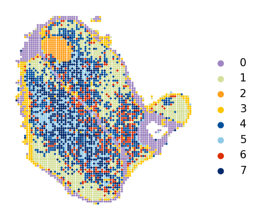
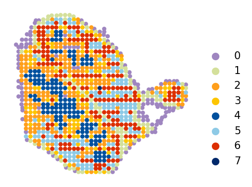
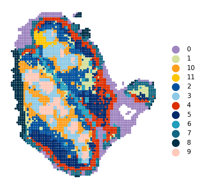
Step 3: (Optional) Visualize Input Data
Before running CORAL, inspect the spatial organization of both modalities. The high-resolution data (CODEX) captures protein expression at single-cell resolution, while the low-resolution data (Visium) measures transcriptomes at a larger spatial scale.
Leiden clustering is used for initial unsupervised visualization. Adjust the res parameter to control cluster granularity.
[5]:
coral.utils.plot_spatial(
    hires_adata,
    res=0.7,
    use_rep_for_cluster='X_pca',
    to_plot_var='cluster',
    need_lognormed=True,
    size=1,
    figsize=(3.5, 3),
    legd=True,
    invert_yaxis=True,
    axis_=False,
    color_list=['#9f86c0', '#d4e09b', '#ff9f1c', '#fdc500', '#00509d', '#8ecae6',
                '#dc2f02', '#00296b', '#219ebc', '#126782', '#023047', '#ffc9b9',
                '#affc41', 'k', 'y', 'g'])
[6]:
coral.utils.plot_spatial(
    lowres_adata,
    res=1.6235,
    use_rep_for_cluster='X_pca',
    to_plot_var='cluster',
    need_lognormed=True,
    size=10,
    figsize=(3.5, 2.7),
    legd=True,
    invert_yaxis=True,
    axis_=False,
    legend_fontsize=10,
    legend_markerscale=2,
    color_list=['#9f86c0', '#d4e09b', '#ff9f1c', '#fdc500', '#00509d', '#8ecae6',
                '#dc2f02', '#00296b', '#219ebc', '#126782', '#023047', '#ffc9b9',
                '#affc41', 'k', 'y', 'g'])
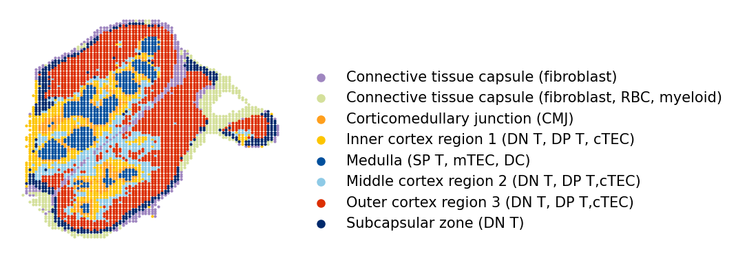
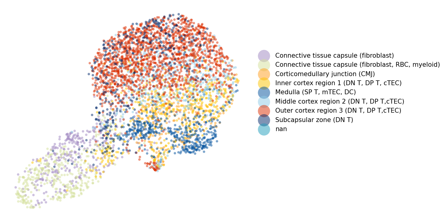
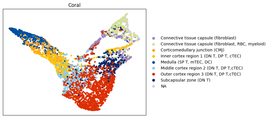
Step 4: (Optional) Visualize Ground Truth Annotations
The ground truth annotations provide manually curated cell-type labels for the high-resolution data. We visualize these in spatial coordinates and as a UMAP embedding to understand the expected tissue organization.
[7]:
coral.utils.plot_spatial(
    ground_truth_adata,
    res=0.7,
    use_rep_for_cluster=None,
    to_plot_var='Annotation',
    need_lognormed=False,
    size=1,
    figsize=(3.5, 3),
    legd=True,
    invert_yaxis=True,
    axis_=False,
    color_list=['#9f86c0', '#d4e09b', '#ff9f1c', '#fdc500', '#00509d', '#8ecae6',
                '#dc2f02', '#00296b', '#219ebc', '#126782', '#023047', '#ffc9b9',
                '#affc41', 'k', 'y', 'g'])
/oak/stanford/groups/quake/siyu/coral_revision2/CORAL/coral/utils/visualization.py:135: UserWarning: Tight layout not applied. The left and right margins cannot be made large enough to accommodate all Axes decorations.
  plt.tight_layout()
[8]:
coral.utils.plot_umap(
    hires_adata,
    res=0.7,
    use_rep_for_cluster='X_pca',
    to_plot_var='Annotation',
    need_lognormed=True,
    size=15,
    figsize=(10, 5),
    legd=True,
    invert_yaxis=True,
    axis_=False,
    color_list=['#9f86c0', '#d4e09b', '#ff9f1c', '#fdc500', '#00509d', '#8ecae6',
                '#dc2f02', '#00296b', '#219ebc', '#126782', '#023047', '#ffc9b9',
                '#affc41', 'k', 'y', 'g'])
[9]:
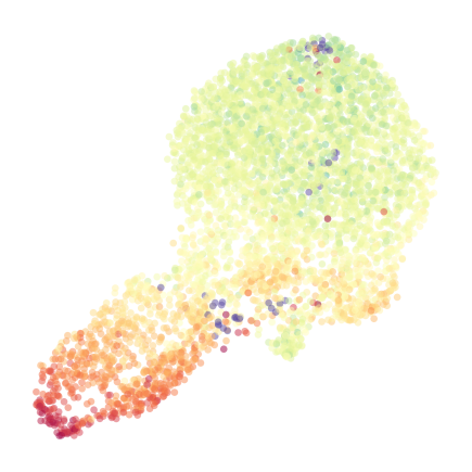
coral.utils.plot_umap_gene(
    hires_adata,
    res=0.7,
    use_rep_for_cluster='X_pca',
    to_plot_gene='Mouse-CD19',
    need_lognormed=True,
    size=10,
    figsize=(3, 3),
    legd=True,
    invert_yaxis=True,
    axis_=False,
    vmin=0,
    vmax=6)
/oak/stanford/groups/quake/siyu/coral_revision2/CORAL/coral/utils/visualization.py:358: UserWarning: No artists with labels found to put in legend.  Note that artists whose label start with an underscore are ignored when legend() is called with no argument.
  ax.legend(
Step 5: Assign Cell Types to High-Resolution Data
CORAL requires cell-type labels for the high-resolution data, used as conditioning variables during training. Here we use Leiden clustering as a proxy for cell types.
Key parameters:
res: Leiden clustering resolution. Higher values produce more clusters. Adjust based on expected number of cell types in your data.use_rep_for_cluster: Representation used for computing the neighbor graph (e.g.,'X_pca').
Note: If manual annotations are available, use those instead of unsupervised clusters for better results.
[10]:
hires_adata = coral.utils.add_cluster(
    hires_adata,
    res=0.7,
    use_rep_for_cluster='X_pca',
    need_lognormed=True)

hires_adata.obs['cell_type'] = hires_adata.obs['cluster']
Step 6: Prepare Data for CORAL
This step preprocesses the input data and constructs local spatial subgraphs for training:
``preprocess_data`` aligns high-resolution cells to their nearest low-resolution spots, concatenates expression matrices, and computes one-hot encoded cell-type vectors.
``prepare_local_subgraphs`` builds k-nearest-neighbor spatial graphs where each subgraph is centered on a high-resolution cell and its local neighborhood.
Key parameters:
n_neighbors: Number of spatial neighbors for graph construction (default: 40). Increase for denser tissues; decrease for sparser ones.
[11]:
combined_expr, hires_coords, one_hot_cell_types, spot_indices, lowres_expr = coral.utils.preprocess_data(
    lowres_adata, hires_adata)

dataloader = coral.utils.prepare_local_subgraphs(
    combined_expr, hires_coords, one_hot_cell_types,
    spot_indices, lowres_expr, n_neighbors=40)
/oak/stanford/groups/quake/siyu/coral_revision2/CORAL/coral/utils/preprocessing.py:130: UserWarning: 'data.DataLoader' is deprecated, use 'loader.DataLoader' instead
  dataloader = DataLoader(data_list, batch_size=8, shuffle=True)
Step 7: Create CORAL Model
Initialize the CORAL model architecture. The model consists of:
Separate encoders for high-resolution (protein) and low-resolution (RNA) modalities
Graph Attention Network (GAT) layers for spatial context encoding
Cross-attention between modalities
Variational inference with latent variables z (shared embedding) and v (nuisance)
Deconvolution layer for cell-type aware expression reconstruction
Key parameters:
latent_dim: Dimension of the shared latent space (default: 64). Larger values capture more variation.hidden_channels: Hidden layer width in GAT (default: 128).v_dim: Dimension of the nuisance variable v (default: 1).
[12]:
device = torch.device('cuda' if torch.cuda.is_available() else 'cpu')

if torch.cuda.is_available():
    print("GPU is available.")
    gpu_count = torch.cuda.device_count()
    print(f"Number of GPUs available: {gpu_count}")
    for i in range(gpu_count):
        print(f"GPU {i}: {torch.cuda.get_device_name(i)}")
else:
    print("GPU is not available. Training will be slower.")
GPU is available.
Number of GPUs available: 1
GPU 0: NVIDIA L40S
[13]:
model, optimizer = coral.model.create_model(
    lowres_dim=lowres_adata.shape[1],
    hires_dim=hires_adata.shape[1],
    lowres_size=lowres_adata.shape[0],
    hires_size=hires_adata.shape[0],
    cell_type_dim=one_hot_cell_types.shape[1],
    latent_dim=64,
    hidden_channels=128,
    v_dim=1)

model.to(device)
[13]:
CORAL_model(
  (encoder_visium): Sequential(
    (0): Linear(in_features=3036, out_features=128, bias=True)
    (1): ReLU()
    (2): Linear(in_features=128, out_features=128, bias=True)
  )
  (encoder_codex): Sequential(
    (0): Linear(in_features=51, out_features=128, bias=True)
    (1): ReLU()
    (2): Linear(in_features=128, out_features=128, bias=True)
  )
  (encoder): Sequential(
    (0): Linear(in_features=3087, out_features=128, bias=True)
    (1): ReLU()
    (2): Linear(in_features=128, out_features=128, bias=True)
  )
  (zi_prior): Sequential(
    (0): Linear(in_features=9, out_features=128, bias=True)
    (1): ReLU()
    (2): Linear(in_features=128, out_features=128, bias=True)
  )
  (cross_attention): CrossAttentionLayer(
    (query_proj): Linear(in_features=64, out_features=64, bias=True)
    (key_proj): Linear(in_features=64, out_features=64, bias=True)
    (value_proj): Linear(in_features=64, out_features=64, bias=True)
    (softmax): Softmax(dim=-1)
  )
  (deconv): DeconvolutionLayer(
    (fc1): Sequential(
      (0): Linear(in_features=3036, out_features=256, bias=True)
      (1): ReLU()
    )
    (fc2): Sequential(
      (0): Linear(in_features=264, out_features=64, bias=True)
      (1): ReLU()
    )
    (fc3): Sequential(
      (0): Linear(in_features=72, out_features=3028, bias=True)
    )
  )
  (gat1): GATConv(64, 128, heads=4)
  (gat2): GATConv(512, 64, heads=1)
  (hidden_decoder): Sequential(
    (0): Linear(in_features=64, out_features=128, bias=True)
    (1): ReLU()
  )
  (visium_scale_decoder): Sequential(
    (0): Linear(in_features=128, out_features=3028, bias=True)
    (1): Softmax(dim=-1)
  )
  (codex_scale_decoder): Sequential(
    (0): Linear(in_features=128, out_features=51, bias=True)
    (1): Softmax(dim=-1)
  )
  (cell_type_decoder): Linear(in_features=64, out_features=8, bias=True)
  (v_layer): Sequential(
    (0): Linear(in_features=3151, out_features=2, bias=True)
  )
  (layer_norm): LayerNorm((512,), eps=1e-05, elementwise_affine=True)
)
Step 8: Train the Model
Train the CORAL model using the prepared dataloader. The loss function includes:
Reconstruction losses (Negative Binomial for RNA, Gamma for protein)
KL divergence for latent variables z and v
Contrastive loss for cross-modal alignment
Graph Laplacian regularization for spatial smoothness
Key parameters:
epochs: Number of training epochs (100 is sufficient for this dataset). Larger or more complex datasets may need 200–300 epochs.
Training progress is printed as per-epoch loss values. Expect the loss to decrease and stabilize.
[14]:
coral.trainer.train_model(model, optimizer, dataloader, epochs=100, device=device)
Epoch 0, Loss: 837648.2199192176
Epoch 1, Loss: 770600.6042729592
Epoch 2, Loss: 769010.3569302721
Epoch 3, Loss: 764302.1369047619
Epoch 4, Loss: 755389.097045068
Epoch 5, Loss: 751568.6720875851
Epoch 6, Loss: 749459.8980654762
Epoch 7, Loss: 746559.7425595238
Epoch 8, Loss: 743714.9146471089
Epoch 9, Loss: 741162.9977678572
Epoch 10, Loss: 737855.4700255102
Epoch 11, Loss: 736055.4667304421
Epoch 12, Loss: 733669.338010204
Epoch 13, Loss: 732623.9071534864
Epoch 14, Loss: 730118.5675488946
Epoch 15, Loss: 729105.441007653
Epoch 16, Loss: 728115.1469494047
Epoch 17, Loss: 727401.9322385204
Epoch 18, Loss: 726170.8336522109
Epoch 19, Loss: 724401.5826955782
Epoch 20, Loss: 723805.8459821428
Epoch 21, Loss: 723725.2316113946
Epoch 22, Loss: 722557.526732568
Epoch 23, Loss: 721548.0806760204
Epoch 24, Loss: 720808.6958971089
Epoch 25, Loss: 720161.651732568
Epoch 26, Loss: 719568.8601190476
Epoch 27, Loss: 718295.4977678572
Epoch 28, Loss: 717804.932557398
Epoch 29, Loss: 717273.8060693027
Epoch 30, Loss: 716792.2909757653
Epoch 31, Loss: 716288.1220769557
Epoch 32, Loss: 715711.6037946428
Epoch 33, Loss: 714526.839445153
Epoch 34, Loss: 714121.5965136054
Epoch 35, Loss: 713558.3742559524
Epoch 36, Loss: 713330.1468431122
Epoch 37, Loss: 712683.857514881
Epoch 38, Loss: 712326.7147108844
Epoch 39, Loss: 711969.3469919218
Epoch 40, Loss: 711465.504517432
Epoch 41, Loss: 710486.9482355443
Epoch 42, Loss: 710597.8776041666
Epoch 43, Loss: 709818.9545068027
Epoch 44, Loss: 709582.885682398
Epoch 45, Loss: 709710.8568239796
Epoch 46, Loss: 708549.2510629252
Epoch 47, Loss: 708097.0718537415
Epoch 48, Loss: 707994.214232568
Epoch 49, Loss: 707722.2387861394
Epoch 50, Loss: 707143.3936011905
Epoch 51, Loss: 705986.8757174745
Epoch 52, Loss: 706633.607727466
Epoch 53, Loss: 706494.7150829082
Epoch 54, Loss: 705708.3996598639
Epoch 55, Loss: 705421.2085990646
Epoch 56, Loss: 705082.2677508503
Epoch 57, Loss: 705406.5555378401
Epoch 58, Loss: 704634.9231505102
Epoch 59, Loss: 703941.4077380953
Epoch 60, Loss: 703309.693877551
Epoch 61, Loss: 703523.401307398
Epoch 62, Loss: 703455.8370535715
Epoch 63, Loss: 703694.8216411564
Epoch 64, Loss: 702864.1707057824
Epoch 65, Loss: 702620.9246386054
Epoch 66, Loss: 702163.7953869047
Epoch 67, Loss: 701483.1818664966
Epoch 68, Loss: 701541.1160182824
Epoch 69, Loss: 701554.693239796
Epoch 70, Loss: 701108.1917517007
Epoch 71, Loss: 701432.1580569728
Epoch 72, Loss: 700882.9892113095
Epoch 73, Loss: 700531.0188137755
Epoch 74, Loss: 700641.3247767857
Epoch 75, Loss: 700588.3956207483
Epoch 76, Loss: 699904.7764136905
Epoch 77, Loss: 699393.0931653911
Epoch 78, Loss: 699899.7037096089
Epoch 79, Loss: 699573.5115858844
Epoch 80, Loss: 698955.6551339285
Epoch 81, Loss: 699121.020567602
Epoch 82, Loss: 699011.3737244898
Epoch 83, Loss: 698875.1813881802
Epoch 84, Loss: 697701.51953125
Epoch 85, Loss: 698005.686065051
Epoch 86, Loss: 697762.2056760204
Epoch 87, Loss: 697990.8284438775
Epoch 88, Loss: 697563.9250106292
Epoch 89, Loss: 697942.4004039116
Epoch 90, Loss: 697859.4511054421
Epoch 91, Loss: 697140.1315901361
Epoch 92, Loss: 697117.7203443878
Epoch 93, Loss: 697276.2634991497
Epoch 94, Loss: 696621.3144664116
Epoch 95, Loss: 697550.0183354592
Epoch 96, Loss: 696702.178039966
Epoch 97, Loss: 696888.1509353742
Epoch 98, Loss: 696591.068664966
Epoch 99, Loss: 696447.1512011054
[15]:
model_save_path = "model.pth"
optimizer_save_path = "optimizer.pth"

torch.save(model.state_dict(), model_save_path)
torch.save(optimizer.state_dict(), optimizer_save_path)
print(f"Model saved to {model_save_path}")
Model saved to model.pth
Step 9: (Optional) Load Pre-trained Model
If you have previously trained a model, you can load it here instead of retraining.
[16]:
model_save_path = "model.pth"
optimizer_save_path = "optimizer.pth"

model.load_state_dict(torch.load(model_save_path))
optimizer.load_state_dict(torch.load(optimizer_save_path))
print("Model loaded successfully.")
Model loaded successfully.
Step 10: Run Inference
Run the trained model on all subgraphs to generate:
CORAL embeddings (
adata.obsm['coral']): Unified latent representation integrating both modalitiesGenerated expression (
adata.obsm['generated_expr']): Deconvolved low-resolution RNA expression at single-cell resolutionEdge indices and attention weights: Graph structure and learned spatial attention for downstream analysis
The output AnnData object is reindexed to match the original high-resolution data ordering.
[17]:
adata_model_gener, edges_all, attn_weights_all = coral.inference.generate_and_validate(
    model, dataloader, device, hires_adata)

adata_model_gener
[17]:
AnnData object with n_obs × n_vars = 4697 × 51
    obsm: 'generated_expr', 'coral', 'spatial', 'v_values', 'cell_types'
Step 11: Analyze CORAL Embeddings
Evaluate the quality of CORAL’s learned embeddings by:
Spatial cluster plot: Leiden clustering on CORAL embeddings, plotted in tissue coordinates
UMAP visualization: CORAL embedding UMAP colored by ground truth annotations
Mutual Information (MI): Quantitative measure of clustering agreement with ground truth (higher = better agreement)
[18]:
# Spatial clusters from CORAL embeddings
coral.utils.plot_spatial(
    adata_model_gener,
    res=0.82,
    use_rep_for_cluster='coral',
    to_plot_var='cluster',
    need_lognormed=True,
    size=5,
    figsize=(4.5, 4.2),
    legd=True,
    invert_yaxis=True,
    axis_=False,
    color_list=['#9f86c0', '#d4e09b', '#ff9f1c', '#fdc500', '#00509d', '#8ecae6',
                '#dc2f02', '#00296b', '#219ebc', '#126782', '#023047', '#ffc9b9',
                '#affc41', 'k', 'y', 'g'])
[19]:
# Add ground truth annotations to the inference output
adata_model_gener.obs['Annotation'] = hires_adata.obs['Annotation'].values

# UMAP of CORAL latent embeddings colored by ground truth annotations
coral.utils.plot_latent_umap(
    adata_model_gener,
    rep='coral',
    to_plot_var='Annotation',
    custom_palette=['#9f86c0', '#d4e09b', '#ff9f1c', '#fdc500', '#00509d', '#8ecae6',
                    '#dc2f02', '#00296b', '#219ebc', '#126782', '#023047', '#ffc9b9',
                    '#affc41', 'k', 'y', 'g'])
/home/users/siyuhe/.local/lib/python3.12/site-packages/umap/umap_.py:1952: UserWarning: n_jobs value 1 overridden to 1 by setting random_state. Use no seed for parallelism.
  warn(
<Figure size 510x450 with 0 Axes>
[20]:
# Compute CORAL embedding clusters using Leiden
adata_eval = adata_model_gener.copy()
sc.pp.neighbors(adata_eval, n_neighbors=100, use_rep='coral')
sc.tl.leiden(adata_eval, resolution=0.82, random_state=0, flavor='igraph')

# Mutual Information: CORAL clusters vs ground truth annotations
mi = mutual_info_score(adata_eval.obs['Annotation'].astype('str'), adata_eval.obs['leiden'])
print(f"Mutual Information (CORAL clusters vs ground truth): {mi:.4f}")
Mutual Information (CORAL clusters vs ground truth): 1.0604
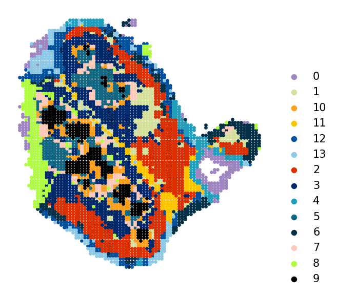
Step 12: Enriched Low-Resolution Data
CORAL produces deconvolved gene expression profiles at single-cell resolution from the low-resolution modality. The generated_expr field in adata_model_gener.obsm contains these enriched profiles — effectively “super-resolving” the Visium spots into individual cell-level RNA expression estimates.
Below we create a standalone AnnData from these enriched profiles and visualize its spatial clusters.
[21]:
# Create AnnData from deconvolved expression
enriched_lowres_adata = anndata.AnnData(adata_model_gener.obsm['generated_expr'])
enriched_lowres_adata.obsm = adata_model_gener.obsm.copy()

# Add gene names from the original low-resolution data if dimensions match
if enriched_lowres_adata.shape[1] <= lowres_adata.shape[1]:
    enriched_lowres_adata.var_names = lowres_adata.var_names[:enriched_lowres_adata.shape[1]].copy()

print(f"Enriched low-resolution AnnData: {enriched_lowres_adata.shape[0]} cells x {enriched_lowres_adata.shape[1]} genes")
Enriched low-resolution AnnData: 4697 cells x 3028 genes
[22]:
coral.utils.plot_spatial(
    enriched_lowres_adata,
    res=1.3,
    use_rep_for_cluster='X_pca',
    to_plot_var='cluster',
    need_lognormed=True,
    size=5,
    figsize=(4.5, 4.2),
    legd=True,
    invert_yaxis=True,
    axis_=False,
    legend_fontsize=10,
    legend_markerscale=2,
    color_list=['#9f86c0', '#d4e09b', '#ff9f1c', '#fdc500', '#00509d', '#8ecae6',
                '#dc2f02', '#00296b', '#219ebc', '#126782', '#023047', '#ffc9b9',
                '#affc41', 'k', 'y', 'g'])
[ ]:
[ ]:
[ ]: